Parallelizing analysis
As we approach the exascale barrier, researchers are handling increasingly large volumes of molecular dynamics (MD) data. Whilst MDAnalysis is a flexible and relatively fast framework for complex analysis tasks in MD simulations, implementing a parallel computing framework would play a pivotal role in accelerating the time to solution for such large datasets.
This document illustrates how you can run your own analysis scripts in parallel with MDAnalysis.
Last executed: Mar 1st, 2022 with MDAnalysis 2.0.0
Last updated: March 2022
Minimum version of MDAnalysis: 2.0.0
Packages required:
MDAnalysisData
dask (https://dask.org/)
dask.distributed (https://distributed.dask.org/en/latest/)
[1]:
import MDAnalysis as mda
from MDAnalysisData.adk_equilibrium import fetch_adk_equilibrium

import numpy as np
import pandas as pd
import matplotlib.pyplot as plt
%matplotlib inline

from multiprocessing import cpu_count
n_jobs = cpu_count()
Background
In MDAnalysis, most implemented analysis methods are based on AnalysisBase, which provides a generic API for users to write their own trajectory analysis. However, this framework only takes single-core power of the PC by iterating through the trajectory and running a frame-wise analysis. Below we aim to first explore some possible simple implementations of parallelism, including using multiprocessing and dask. We will also discuss the acceleration approaches that should be considered,
ranging from your own multiple-core laptops/desktops to distributed clusters. “
Loading files
The test files we will be working with here feature adenylate kinase (AdK), a phosopho-transferase enzyme. ([BDPW09]). The trajectory has 4187 frames, which will take quite some time to run the analysis on with the conventional serial (single-core) approach.
Note: downloading these datasets from MDAnalysisData may take some time.
[2]:
adk = fetch_adk_equilibrium()
u = mda.Universe(adk.topology, adk.trajectory)
protein = u.select_atoms('protein')
[3]:
u.trajectory
[3]:
<DCDReader /home/scottzhuang/MDAnalysis_data/adk_equilibrium/1ake_007-nowater-core-dt240ps.dcd with 4187 frames of 3341 atoms>
Radius of gyration
For a detail description of this analysis, read Writing your own trajectory.
Here is a common form of single-frame method that we can normally see inside AnalysisBase. It may contain both some dynamic parts that changes along time either implicitly or explicitly (e.g. AtomGroup) and some static parts (e.g. a reference frame).
[4]:
def radgyr(atomgroup, masses, total_mass=None):
    # coordinates change for each frame
    coordinates = atomgroup.positions
    center_of_mass = atomgroup.center_of_mass()

    # get squared distance from center
    ri_sq = (coordinates-center_of_mass)**2
    # sum the unweighted positions
    sq = np.sum(ri_sq, axis=1)
    sq_x = np.sum(ri_sq[:,[1,2]], axis=1) # sum over y and z
    sq_y = np.sum(ri_sq[:,[0,2]], axis=1) # sum over x and z
    sq_z = np.sum(ri_sq[:,[0,1]], axis=1) # sum over x and y

    # make into array
    sq_rs = np.array([sq, sq_x, sq_y, sq_z])

    # weight positions
    rog_sq = np.sum(masses*sq_rs, axis=1)/total_mass
    # square root and return
    return np.sqrt(rog_sq)
Serial Analysis
Below is the serial version of the analysis that we normally use.
[5]:
result = []
for frame in u.trajectory:
    result.append(radgyr(atomgroup=protein,
                         masses=protein.masses,
                         total_mass=np.sum(protein.masses)))
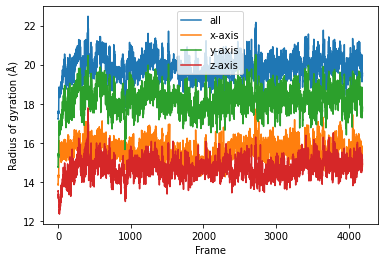
[6]:
result = np.asarray(result).T

labels = ['all', 'x-axis', 'y-axis', 'z-axis']
for col, label in zip(result, labels):
    plt.plot(col, label=label)
plt.legend()
plt.ylabel('Radius of gyration (Å)')
plt.xlabel('Frame');

Parallelization in a simple per-frame fashion
Frame-wise form of the function
The coordinates of the atomgroup analysed change with each frame of the trajectory. We need to explicitly point the analysis function to the frame that needs to be analysed with a frame_index: atomgroup.universe.trajectory[frame_index] in order to update the positions (and any other dynamic per-frame information) appropriately. Therefore, the first step to making the radgyr function parallelisable is to add a frame_index argument.
[7]:
def radgyr_per_frame(frame_index, atomgroup, masses, total_mass=None):

    # index the trajectory to set it to the frame_index frame
    atomgroup.universe.trajectory[frame_index]

    # coordinates change for each frame
    coordinates = atomgroup.positions
    center_of_mass = atomgroup.center_of_mass()

    # get squared distance from center
    ri_sq = (coordinates-center_of_mass)**2
    # sum the unweighted positions
    sq = np.sum(ri_sq, axis=1)
    sq_x = np.sum(ri_sq[:,[1,2]], axis=1) # sum over y and z
    sq_y = np.sum(ri_sq[:,[0,2]], axis=1) # sum over x and z
    sq_z = np.sum(ri_sq[:,[0,1]], axis=1) # sum over x and y

    # make into array
    sq_rs = np.array([sq, sq_x, sq_y, sq_z])

    # weight positions
    rog_sq = np.sum(masses*sq_rs, axis=1)/total_mass
    # square root and return
    return np.sqrt(rog_sq)
Parallelization with multiprocessing
The native parallelisation module in Python is called multiprocessing. It contains useful tools to build a pool of working cores, map the function into different workers, and gather and order the results from all the workers.
Below we use Pool from multiprocessing as a context manager. We can define how many cores (or workers) we want to use with Pool(n_jobs).
[8]:
import multiprocessing
from multiprocessing import Pool
from functools import partial
We use functools.partial to create a new method by supplying every argument needed for radgyr_per_frame except frame_index. We can do this because the atomgroup, masses etc. will not change when we iterate the function over each frame, but the frame_index will. We create a list of jobs where we use the worker_pool to map each frame_index to each job.
[9]:
run_per_frame = partial(radgyr_per_frame,
                        atomgroup=protein,
                        masses=protein.masses,
                        total_mass=np.sum(protein.masses))

frame_values = np.arange(u.trajectory.n_frames)
[10]:
with Pool(n_jobs) as worker_pool:
    result = worker_pool.map(run_per_frame, frame_values)
The result will be a list of arrays containing the result for each frame. Finally the results can be plotted along time.
[11]:
result = np.asarray(result).T

labels = ['all', 'x-axis', 'y-axis', 'z-axis']
for col, label in zip(result, labels):
    plt.plot(col, label=label)
plt.legend()
plt.ylabel('Radius of gyration (Å)')
plt.xlabel('Frame');

Parallelization with dask
Dask is a flexible library for parallel computing in Python. It provides advanced parallelism for analytics and has been integrated or utilized in many scientific softwares. It can be scaled from one single computer to a cluster of computers inside a HPC center.
Dask has a dynamic task scheduling system with synchronous (single-threaded), threaded, multiprocessing and distributed schedulers. The wrapping function in dask, dask.delayed, mimics for loops and wraps Python code into a Dask graph. This code can then be easily run in parallel, and visualized with dask.visualize() to examine if the task is well distributed. The code inside dask.delayed is not run immediately on execution, but pushed into a job queue waiting for submission. You can
read more on dask website.
Comaring to multiprocssing, the downside of multiprocessing is that it is mostly focused on single-machine multicore parallelism (without extra manager). It is hard to operate on multimachine conditions. Below are two simple examples to use Dask to achieve the same task as multiprocessing does.
The API of dask is similar to multiprocessing. It also creates a pool of workers for your single machine with the given resources.
Note: The threaded scheduler in Dask (similar to threading in Python) should not be used as it will mess up with the state (timestep) of the trajectory.
[12]:
import dask
import dask.multiprocessing
dask.config.set(scheduler='processes')
[12]:
<dask.config.set at 0x7f4768417280>
Below is how you can utilize dask.distributed module to build a local cluster.
Note: this is not really needed for your laptop/desktop. Using dask.distributed may even slow down the performance, but it provides a diagnostic dashboard that can provide valuable insight on performance and progress.
See limitations here: https://distributed.dask.org/en/latest/limitations.html
[13]:
from dask.distributed import Client

client = Client(n_workers=n_jobs)
client
[13]:
Client
|
Cluster
|
First we have to create a list of jobs and transform them with dask.delayed() so they can be processed by Dask.
[14]:
job_list = []
for frame_index in range(u.trajectory.n_frames):
    job_list.append(dask.delayed(radgyr_per_frame(frame_index,
                                        atomgroup=protein,
                                        masses=protein.masses,
                                        total_mass=np.sum(protein.masses))))
Then we simply use dask.compute() to get a list of ordered results.
[15]:
result = dask.compute(job_list)
[16]:
result = np.asarray(result).T

labels = ['all', 'x-axis', 'y-axis', 'z-axis']
for col, label in zip(result, labels):
    plt.plot(col, label=label)
plt.legend()
plt.ylabel('Radius of gyration (Å)')
plt.xlabel('Frame');

We can also use the old radgyr function because dask is more flexible on the input arguments.
Note: the associated timestamp of protein will change during the trajectory iteration, so the processes are always aware which timestep the trajectory is in and change the protein (e.g. its coordinates) accordingly.
[17]:
job_list = []
for frame in u.trajectory:
    job_list.append(dask.delayed(radgyr(atomgroup=protein,
                                        masses=protein.masses,
                                        total_mass=np.sum(protein.masses))))
Then we simply use dask.compute() to get a list of ordered results.
[18]:
result = dask.compute(job_list)
[19]:
result = np.asarray(result).T

labels = ['all', 'x-axis', 'y-axis', 'z-axis']
for col, label in zip(result, labels):
    plt.plot(col, label=label)
plt.legend()
plt.ylabel('Radius of gyration (Å)')
plt.xlabel('Frame');
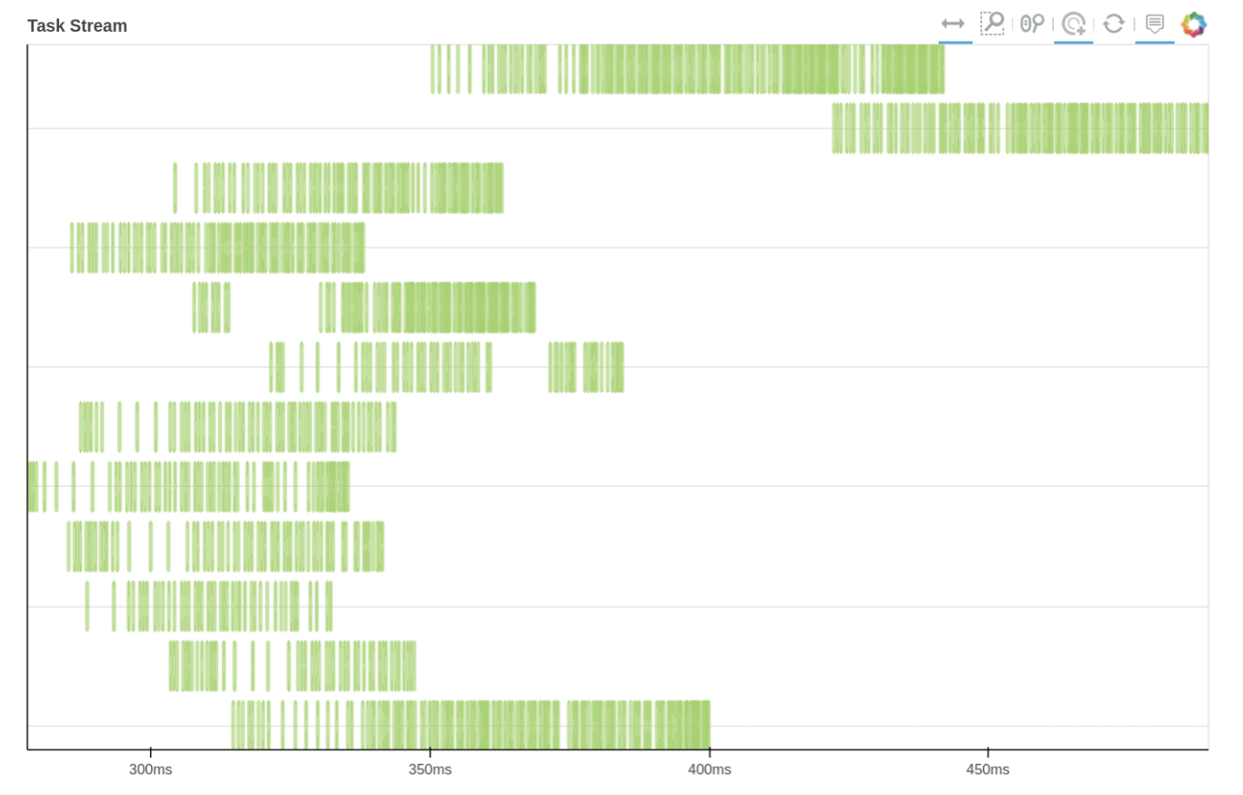
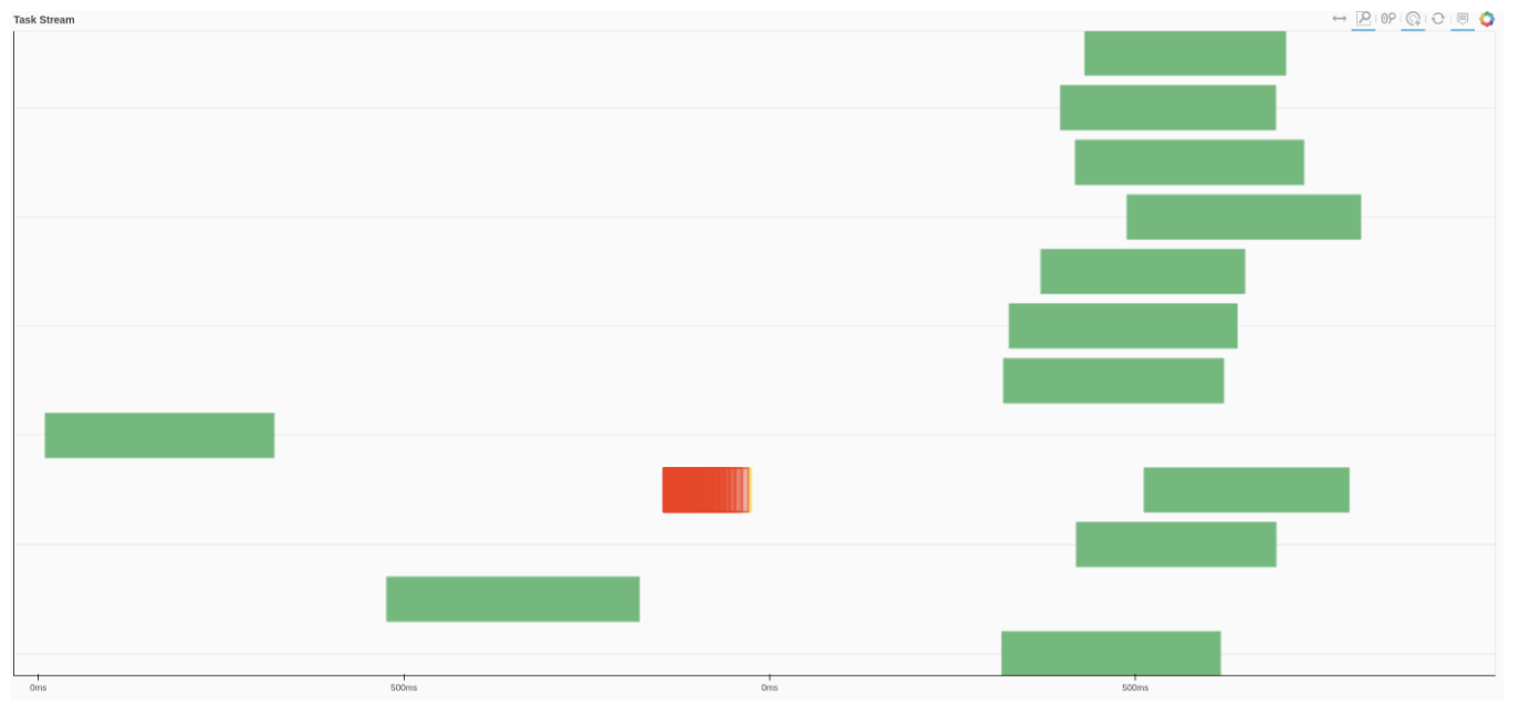
We can also use Dask dashboard (with dask.distributed.Client) to examine how jobs are distributed along all the workers. Each green bar below represents one job, i.e. running radgyr on one frame of the trajectory
Parallelization in a split-apply-combine fashion
The aforementioned per-frame approach should normally be avoided because in each task, all the attributes (AtomGroup, Universe, and etc) need to be pickled. This pickling may take even more time than your lightweight analysis! Besides, in Dask, a significant amount of overhead time is needed to build a comprehensive Dask graph with thousands of tasks.
Therefore, we should normally use a split-apply-combine scheme for parallel trajectory analysis. Here, the trajectory is split into blocks, analysis is performed separately and in parallel on each block (“apply”), and then results from each block are gathered and combined.
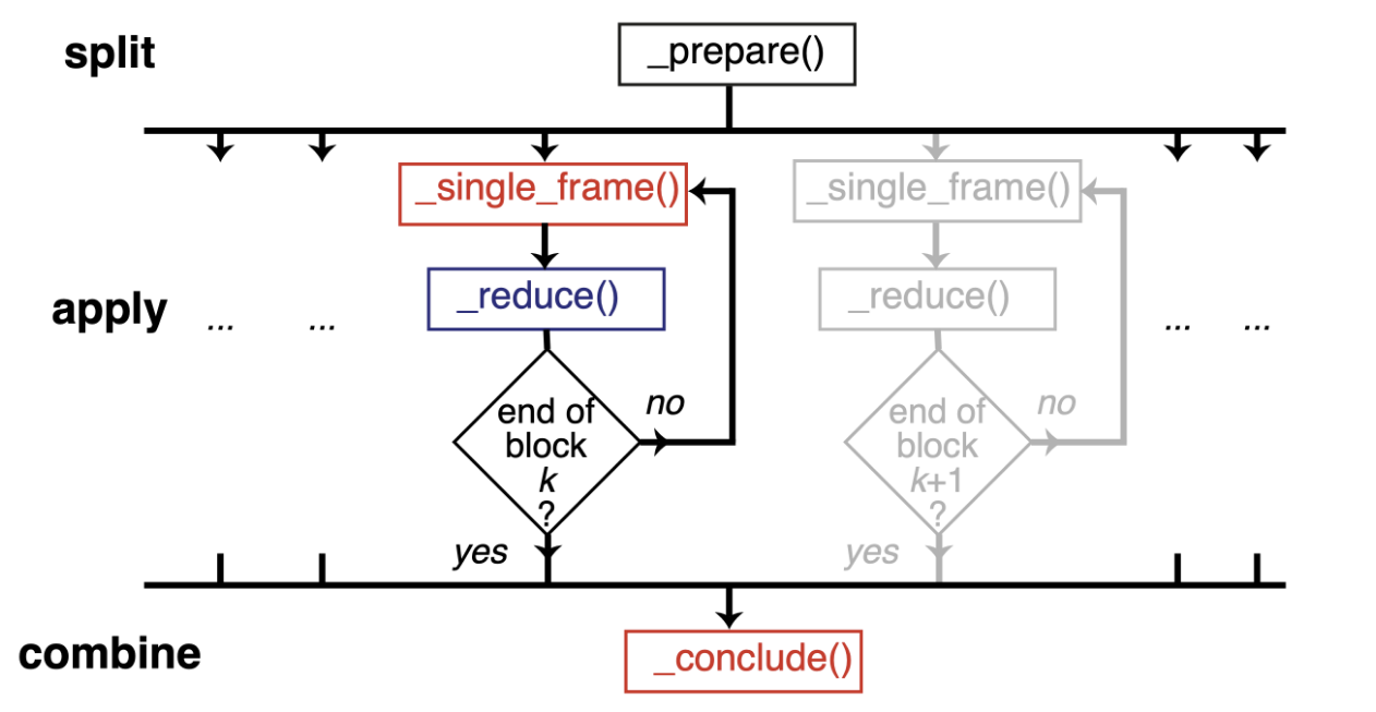
Image from ([SFPG+19]) used under CC-BY license.
We will show a simple illustration of split-apply-combine approach with dask below:
Block analysis function
@dask.delayed is a common syntax to decorate a function into delayed-enabled. It is the same as delaying the function by dask.delayed(analyze_block)(bs, radgyr, ...) later on.
[20]:
@dask.delayed
def analyze_block(blockslice, func, *args, **kwargs):
    result = []
    for ts in u.trajectory[blockslice.start:blockslice.stop]:
        A = func(*args, **kwargs)
        result.append(A)
    return result
Split the trajectory
This is a very simple way to split the trajectory. It splits the trajectory into defined n_blocks which is normally the same as the number of cores you want to use.
Since it is achieved by evenly dividing the n_frames by n_blocks, and setting the last block to end at the last frame, sometime it is not really balanced (e.g. the last block).
[21]:
n_frames = u.trajectory.n_frames
n_blocks = n_jobs   #  it can be any realistic value (0 < n_blocks <= n_jobs)

n_frames_per_block = n_frames // n_blocks
blocks = [range(i * n_frames_per_block, (i + 1) * n_frames_per_block) for i in range(n_blocks-1)]
blocks.append(range((n_blocks - 1) * n_frames_per_block, n_frames))
[22]:
blocks
[22]:
[range(0, 348),
 range(348, 696),
 range(696, 1044),
 range(1044, 1392),
 range(1392, 1740),
 range(1740, 2088),
 range(2088, 2436),
 range(2436, 2784),
 range(2784, 3132),
 range(3132, 3480),
 range(3480, 3828),
 range(3828, 4187)]
Apply the analysis per block
[23]:
jobs = []
for bs in blocks:
    jobs.append(analyze_block(bs,
                              radgyr,
                              protein,
                              protein.masses,
                              total_mass=np.sum(protein.masses)))
jobs = dask.delayed(jobs)
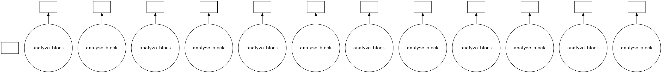
Using visualize() we can see that the trajectory is split into a few blocks instead of ~4000 jobs.
[24]:
jobs.visualize()
[24]:
[25]:
results = jobs.compute()
Combine the results
[26]:
result = np.concatenate(results)
[27]:
result = np.asarray(result).T

labels = ['all', 'x-axis', 'y-axis', 'z-axis']
for col, label in zip(result, labels):
    plt.plot(col, label=label)
plt.legend()
plt.ylabel('Radius of gyration (Å)')
plt.xlabel('Frame');

If you look at the Dask dashboard (with dask.distributed.Client) this time, you will see each green bar below represents a per-block analysis for radgyr.
Other possible parallelism approaches for multiple analyses
You may want to perform multiple analyses (or analyze multiple trajectories). In this case, you can use some high-level parallelism, i.e. running all the serial analyses in parallel.
Here we use joblib. It is implemented on multiprocessing and provides lightweight pipelining in Python. Compared to multiprocessing, it has a simple API and convenient persistence of cached results.”
[28]:
from joblib import Parallel, delayed
import multiprocessing
num_cores = multiprocessing.cpu_count()
Here we leverage the power of AnalysisFromFunction to fast construct a class that will iterate through the trajectory and save the analysis results.
If you want to know more about how AnalysisFromFunction works, you can read it from Writing your own trajectory.
[29]:
from MDAnalysis.analysis.base import AnalysisFromFunction
[30]:
rog_1 = AnalysisFromFunction(radgyr, u.trajectory,
                           protein, protein.masses,
                           total_mass=np.sum(protein.masses))

rog_2 = AnalysisFromFunction(radgyr, u.trajectory,
                           protein, protein.masses,
                           total_mass=np.sum(protein.masses))

rog_3 = AnalysisFromFunction(radgyr, u.trajectory,
                           protein, protein.masses,
                           total_mass=np.sum(protein.masses))

rog_4 = AnalysisFromFunction(radgyr, u.trajectory,
                           protein, protein.masses,
                           total_mass=np.sum(protein.masses))

analysis_ensemble = [rog_1, rog_2, rog_3, rog_4]
run_analysis is a simple way to run the analysis and retrieve the results.
[31]:
def run_analysis(analysis):
    analysis.run()
    return analysis.results
The joblib.delayed is different from dask.delayed; it cannot be used as a “pie” syntax (@joblib.delayed), so you have to use it as below.
Similiar to dask.delayed, the code inside joblib.delayed will not run immediately but be pushed into a job queue waiting for processing. In this case, run_anlaysis() is processed by Parallel with defined number of workers–n_jobs.
[32]:
results_ensemble = Parallel(n_jobs=num_cores)(delayed(run_analysis)(analysis)
                                                for analysis in analysis_ensemble)
The results_ensemble will be a list of results that is returned from run_analysis. You can further split and process each analysis.
[33]:
result_1 = np.asarray(results_ensemble[0]['timeseries']).T

labels = ['all', 'x-axis', 'y-axis', 'z-axis']
for col, label in zip(result_1, labels):
    plt.plot(col, label=label)
plt.legend()
plt.ylabel('Radius of gyration (Å)')
plt.xlabel('Frame');

See Also
The parallel version of MDAnalysis is still under development. For existing solutions and some implementations of parallel analysis, go to PMDA. PMDA ([SFPG+19]) applies the aforementioned split-apply-combine scheme with Dask. In the future, it may provide a framework that consolidates all the parallelisation schemes described in this tutorial.”
References
[1] Oliver Beckstein, Elizabeth J. Denning, Juan R. Perilla, and Thomas B. Woolf. Zipping and Unzipping of Adenylate Kinase: Atomistic Insights into the Ensemble of Open↔Closed Transitions. Journal of Molecular Biology, 394(1):160–176, November 2009. 00107. URL: https://linkinghub.elsevier.com/retrieve/pii/S0022283609011164, doi:10.1016/j.jmb.2009.09.009.
[2] Richard J. Gowers, Max Linke, Jonathan Barnoud, Tyler J. E. Reddy, Manuel N. Melo, Sean L. Seyler, Jan Domański, David L. Dotson, Sébastien Buchoux, Ian M. Kenney, and Oliver Beckstein. MDAnalysis: A Python Package for the Rapid Analysis of Molecular Dynamics Simulations. Proceedings of the 15th Python in Science Conference, pages 98–105, 2016. 00152. URL: https://conference.scipy.org/proceedings/scipy2016/oliver_beckstein.html, doi:10.25080/Majora-629e541a-00e.
[3] Naveen Michaud-Agrawal, Elizabeth J. Denning, Thomas B. Woolf, and Oliver Beckstein. MDAnalysis: A toolkit for the analysis of molecular dynamics simulations. Journal of Computational Chemistry, 32(10):2319–2327, July 2011. 00778. URL: http://doi.wiley.com/10.1002/jcc.21787, doi:10.1002/jcc.21787.
[4] Max Linke Shujie Fan, Ioannis Paraskevakos, Richard J. Gowers, Michael Gecht, and Oliver Beckstein. PMDA - Parallel Molecular Dynamics Analysis. In Chris Calloway, David Lippa, Dillon Niederhut, and David Shupe, editors, Proceedings of the 18th Python in Science Conference, 134 – 142. 2019. doi:10.25080/Majora-7ddc1dd1-013.