Calculating hydrogen bonds: the basics
We will find the hydrogen bonds in a box of water in order to demonstrate the basic usage of HydrogenBondAnaysis.
Last updated: June 22, 2021 with MDAnalysis 2.0.0-dev
Minimum version of MDAnalysis: 2.0.0-dev0
Packages required:
MDAnalysisTests
See also
Note
Please cite Smith et al. (2018) when using HydrogenBondAnaysis in published work.
[1]:
import pickle
import numpy as np
np.set_printoptions(linewidth=100)
import pandas as pd

import matplotlib.pyplot as plt

import MDAnalysis as mda
from MDAnalysis.tests.datafiles import waterPSF, waterDCD
from MDAnalysis.analysis.hydrogenbonds import HydrogenBondAnalysis

# the next line is necessary to display plots in Jupyter
%matplotlib inline
Loading files
We will load a small water-only system containing 5 water molecules and 10 frames then find the hydrogen bonds present at each frame.
[2]:
u = mda.Universe(waterPSF, waterDCD)
Warning
It is highly recommended that a topology with bond information is used (e.g. PSF, TPR, PRMTOP), as this is the only way to guarantee the correct identification of donor-hydrogen pairs.
Hydrogen bonds
In molecular dynamics simulations, hydrogen bonds are typically identified via the following geometric criteria:
the donor-acceptor distance (\(r_{DA}\)) must be less than a specified cutoff, typically 3 Å
the donor-hydrogen-acceptor angle (\(\theta_{DHA}\)) must be greater than a specified cutoff, typically 150°

Find water-water hydrogen bonds
Basic usage of HydrogenBondAnalysis involvees passing an acceptor atom selection (acceptors_sel) and a hydrogen atom selection (hydrogens_sel) to HydrogenBondAnalysis. By not providing a donor atom selection (donor_sel) we will use the topology bond information to find donor-hydrogen pairs.
In the following cell, acceptors_sel="name OH2" and hydrogens_sel="name H1 H2" will select the oxygen and hydrogen atoms, respectively, of water. The names correspond to those for the CHARMM TIP3P water model and may be different for other force fields.
[3]:
hbonds = HydrogenBondAnalysis(
    universe=u,
    donors_sel=None,
    hydrogens_sel="name H1 H2",
    acceptors_sel="name OH2",
    d_a_cutoff=3.0,
    d_h_a_angle_cutoff=150,
    update_selections=False
)
Note
For a performance boost, update_selections can be set to False.
However, always set update_selections to True if you think that your selection will update over time. For example, the number of oxygen atoms within 3.0 Å may change over time if you choose acceptors_sel="name OH2 and around 3.0 protein.
See also the MDAnalysis documentation on updating AtomGroups.
We then use the run() method to perform the analysis. If we do not set the start, stop, and step for frames to analyse, all frames will be used.
[4]:
hbonds.run(
    start=None,
    stop=None,
    step=None,
    verbose=True
)
Accessing the results
The results are stored as a numpy array in the hbonds.results.hbonds attribute. The array is of shape \((N_\textrm{hbonds}, 6)\).
[5]:
# We see there are 27 hydrogen bonds in total
print(hbonds.results.hbonds.shape)
(27, 6)
Each row of the results array contains the follwing information on a single hydrogen bond:
[frame, donor_index, hydrogen_index, acceptor_index, DA_distance, DHA_angle]
Let’s take a look at the first hydrogen bond found:
[6]:
print(hbonds.results.hbonds[0])
[ 0. 9. 10. 3. 2.82744082 150.48955173]
This hydrogen bond was found at frame 0. The donor, hydrogen, and acceptor atoms have indices 9, 10, and 3, respectively. There is a distance of 2.83 Å between the donor and acceptor atoms, and an angle of 150° made by the donor-hydrogen-acceptor atoms.
The frame number and atom indices can be used to select the atoms involved in the above hydrogen bond. However, as the results array is of type float64, these values must first be cast to integers:
[7]:
hbonds.results.hbonds.dtype
[7]:
dtype('float64')
[8]:
first_hbond = hbonds.results.hbonds[0]
[9]:
frame, donor_ix, hydrogen_ix, acceptor_ix = first_hbond[:4].astype(int)
[10]:
# select the correct frame and the atoms involved in the hydrogen bond
u.trajectory[frame]
atoms = u.atoms[[donor_ix, hydrogen_ix, acceptor_ix]]
[11]:
atoms
[11]:
<AtomGroup with 3 atoms>
For clarity, below we define constants that will be used throughout the rest of the notebook to access the relevant column of each hbond row
[12]:
FRAME = 0
DONOR = 1
HYDROGEN = 2
ACCEPTOR = 3
DISTANCE = 4
ANGLE = 5
Helper functions
The are three helper functions that can be used to quickly post-process the results.
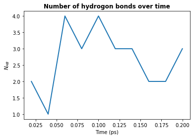
1. Count by time. Counts the total number of hydrogen bonds at each frame
[13]:
plt.plot(hbonds.times, hbonds.count_by_time(), lw=2)

plt.title("Number of hydrogon bonds over time", weight="bold")
plt.xlabel("Time (ps)")
plt.ylabel(r"$N_{HB}$")

plt.show()
2. Count by type. Counts the total number of each type of hydrogen bond.
A type is a unique combination of donor residue name, donor atom type, acceptor residue name, and acceptor atom type.
[14]:
hbonds.count_by_type()
[14]:
array([['TIP3:OT', 'TIP3:OT', '27']], dtype='<U7')
Each row contains a unique hydrogen bond type. The three columns correspond to:
the donor resname and atom name (here, the OT atom of the TIP3 water residue)
the acceptor resname and atom name (here, the OT atom of the TIP3 water residue)
the total count
The average number of each type of hydrogen bond formed at each frame is likely more informative than the total number over the trajectory. This can be calculated for each hydrogen bond type as follows:
[15]:
for donor, acceptor, count in hbonds.count_by_type():

    donor_resname, donor_type = donor.split(":")
    n_donors = u.select_atoms(f"resname {donor_resname} and type {donor_type}").n_atoms

    # average number of hbonds per donor molecule per frame
    mean_count = 2 * int(count) / (hbonds.n_frames * n_donors)  # multiply by two as each hydrogen bond involves two water molecules
    print(f"{donor} to {acceptor}: {mean_count:.2f}")
TIP3:OT to TIP3:OT: 1.08
Note
In a water-only system the average number of hydrogen bonds per water molecule should be around 3.3, depending on temperature and forcefield. We don’t see this due to the small system size (15 water molecules).
3. Count by ids. Counts the total number of each hydrogen bond formed between specific atoms.
[16]:
hbonds.count_by_ids()
[16]:
array([[12, 14,  9, 10],
       [ 9, 10,  3,  9],
       [ 3,  5,  0,  4],
       [ 0,  1,  6,  3],
       [ 6,  7, 12,  1]])
Each row contains a unique hydrogen bond. The four columns correspond to:
the donor atom index
the hydrogen atom index
the acceptor atom index
the total count
The array is sorted in descending total count. You can check which atoms are involved in the most frequently observed hydrogen bond:
[17]:
counts = hbonds.count_by_ids()
most_common = counts[0]

print(f"Most common donor: {u.atoms[most_common[0]]}")
print(f"Most common hydrogen: {u.atoms[most_common[1]]}")
print(f"Most common acceptor: {u.atoms[most_common[2]]}")
Most common donor: <Atom 13: OH2 of type OT of resname TIP3, resid 21 and segid WAT>
Most common hydrogen: <Atom 15: H2 of type HT of resname TIP3, resid 21 and segid WAT>
Most common acceptor: <Atom 10: OH2 of type OT of resname TIP3, resid 15 and segid WAT>
Further analysis
There are many different analyses you may want to perform after finding hydrogen bonds. Below we will calculate the mean number of hydrogen bonds as a function of \(z\) position of the donor atom.
[18]:
# bins in z for the histogram
bin_edges = np.linspace(-25, 25, 51)
bin_centers = bin_edges[:-1] + 0.5

# results array (this is faster and more memory efficient than appending to a list)
counts = np.full(bin_centers.size, fill_value=0.0)
[19]:
for frame, donor_ix, *_ in hbonds.hbonds:

    u.trajectory[frame.astype(int)]
    donor = u.atoms[donor_ix.astype(int)]

    zpos = donor.position[2]
    hist, *_ = np.histogram(zpos, bins=bin_edges)
    counts += hist * 2  # multiply by two as each hydrogen bond involves two water molecules

counts /= hbonds.n_frames
[20]:
plt.plot(bin_centers, counts, lw=2)

plt.title(r"Number of hydrogen bonds as a funcion of height in $z$", weight="bold")
plt.xlabel(r"$z\ \rm (\AA)$")
plt.ylabel(r"$N_{HB}$")

plt.show()
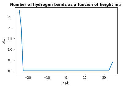
You may wish to find the number of hydrogen bonds in \(z\) per unit area in \(xy\), rather than the total number a each \(z\) position. To do this, simply divide counts by the mean area in \(xy\):
[21]:
mean_xy_area = np.mean(
    [np.product(ts.dimensions[:2]) for ts in u.trajectory[hbonds.frames]]
)
counts /= mean_xy_area
Note
It is likely you will want to calculate the distance from an interface, such as a lipid membrane, rather than the absolute position in \(z\). For example, if you have a bilayer that is centered at 0, you might define your interface as the mean position in \(z\) of the phosphorous atoms in the upper leaflet of the bilayer:
headgroup_atoms = u.select_atoms(“name P”) interface_zpos = np.mean(headgroup_atoms.positions[:, 2])
zpos = donors.positions[:,2] - interface_zpos
Store data
There are various ways of storing the results from the analysis.
You can persist the HydrogenBondsAnalysis object using pickle (or joblib)
[22]:
with open("hbonds.pkl", 'wb') as f:
    pickle.dump(hbonds, f)
[23]:
with open("hbonds.pkl", 'rb') as f:
    hbonds = pickle.load(f)
You can extract the results and store the numpy array
[24]:
np.save("hbonds.npy", hbonds.hbonds)
You can create a Pandas DataFrame with more information about hydrogen bonding atoms, which may make some further analysis easier.
[25]:
df = pd.DataFrame(hbonds.results.hbonds[:, :DISTANCE].astype(int),
                  columns=["Frame",
                           "Donor_ix",
                           "Hydrogen_ix",
                           "Acceptor_ix",])

df["Distances"] = hbonds.results.hbonds[:, DISTANCE]
df["Angles"] = hbonds.results.hbonds[:, ANGLE]

df["Donor resname"] = u.atoms[df.Donor_ix].resnames
df["Acceptor resname"] = u.atoms[df.Acceptor_ix].resnames
df["Donor resid"] = u.atoms[df.Donor_ix].resids
df["Acceptor resid"] = u.atoms[df.Acceptor_ix].resids
df["Donor name"] = u.atoms[df.Donor_ix].names
df["Acceptor name"] = u.atoms[df.Acceptor_ix].names
[26]:
df.to_csv("hbonds.csv", index=False)
References
[1] Richard J. Gowers, Max Linke, Jonathan Barnoud, Tyler J. E. Reddy, Manuel N. Melo, Sean L. Seyler, Jan Domański, David L. Dotson, Sébastien Buchoux, Ian M. Kenney, and Oliver Beckstein. MDAnalysis: A Python Package for the Rapid Analysis of Molecular Dynamics Simulations. Proceedings of the 15th Python in Science Conference, pages 98–105, 2016. 00152. URL: https://conference.scipy.org/proceedings/scipy2016/oliver_beckstein.html, doi:10.25080/Majora-629e541a-00e.
[2] Naveen Michaud-Agrawal, Elizabeth J. Denning, Thomas B. Woolf, and Oliver Beckstein. MDAnalysis: A toolkit for the analysis of molecular dynamics simulations. Journal of Computational Chemistry, 32(10):2319–2327, July 2011. 00778. URL: http://doi.wiley.com/10.1002/jcc.21787, doi:10.1002/jcc.21787.
[3] Paul Smith, Robert M. Ziolek, Elena Gazzarrini, Dylan M. Owen, and Christian D. Lorenz. On the interaction of hyaluronic acid with synovial fluid lipid membranes. Phys. Chem. Chem. Phys., 21(19):9845-9857, 2018. URL: http://dx.doi.org/10.1039/C9CP01532A