Calculating hydrogen bond lifetimes
We will calculate the lifetime of intramolecular hydrogen bonds in a protein.
Last updated: June 23, 2021 with MDAnalysis 2.0.0-dev
Minimum version of MDAnalysis: 2.0.0-dev0
Packages required:
MDAnalysisTests
See also
Note
Please cite Smith et al. (2018) when using HydrogenBondAnaysis in published work.
[1]:
from tqdm.auto import tqdm
import numpy as np
import matplotlib.pyplot as plt

import MDAnalysis as mda
from MDAnalysis.tests.datafiles import PSF, DCD
from MDAnalysis.analysis.hydrogenbonds import HydrogenBondAnalysis
Loading files
[2]:
u = mda.Universe(PSF, DCD)
The test files we will be working with here feature adenylate kinase (AdK), a phosophotransferase enzyme. ([BDPW09])
Find all hydrogen bonds
First, find the hydrogen bonds.
[3]:
hbonds = HydrogenBondAnalysis(universe=u)
[4]:
hbonds.run(verbose=True)
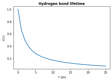
Calculate hydrogen bond lifetimes
The hydrogen bond lifetime is calculated via the time autocorrelation function of the presence of a hydrogen bond:
where \(h_{ij}\) indicates the presence of a hydrogen bond between atoms \(i\) and \(j\):
\(h_{ij}=1\) if there is a hydrogen bond
\(h_{ij}=0\) if there is no hydrogen bond
\(h_{ij}(t_0)=1\) indicates there is a hydrogen bond between atoms \(i\) and \(j\) at a time origin \(t_0\), and \(h_{ij}(t_0+\tau)=1\) indicates these atoms remain hydrogen bonded throughout the period \(t_0\) to \(t_0+\tau\). To improve statistics, multiple time origins, \(t_0\), are used in the calculation and the average is taken over all time origins.
See Gowers and Carbonne (2015) for further discussion on hydrogen bonds lifetimes.
Note
The period between time origins, \(t_0\), should be chosen such that consecutive \(t_0\) are uncorrelated.
The hbonds.lifetime method calculates the above time autocorrelation function. The period between time origins is set using window_step, and the maximum value of \(\tau\) (in frames) is set using tau_max.
[5]:
tau_max = 25
window_step = 1
[6]:
tau_frames, hbond_lifetime = hbonds.lifetime(
    tau_max=tau_max,
    window_step=window_step
)
[7]:
tau_times = tau_frames * u.trajectory.dt
plt.plot(tau_times, hbond_lifetime, lw=2)

plt.title(r"Hydrogen bond lifetime", weight="bold")
plt.xlabel(r"$\tau\ \rm (ps)$")
plt.ylabel(r"$C(\tau)$")

plt.show()
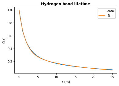
Calculating the time constant
To obtain the hydrogen bond lifetime, you can fit a biexponential to the time autocorrelation curve. We will fit the following biexponential:
where \(\tau_1\) and \(\tau_2\) represent two time constants - one corresponding to a short-timescale process and the other to a longer timescale process. \(A\) and \(B\) will sum to \(1\), and they represent the relative importance of the short- and longer-timescale processes in the overall autocorrelation curve.
[8]:
def fit_biexponential(tau_timeseries, ac_timeseries):
    """Fit a biexponential function to a hydrogen bond time autocorrelation function

    Return the two time constants
    """
    from scipy.optimize import curve_fit

    def model(t, A, tau1, B, tau2):
        """Fit data to a biexponential function.
        """
        return A * np.exp(-t / tau1) + B * np.exp(-t / tau2)

    params, params_covariance = curve_fit(model, tau_timeseries, ac_timeseries, [1, 0.5, 1, 2])

    fit_t = np.linspace(tau_timeseries[0], tau_timeseries[-1], 1000)
    fit_ac = model(fit_t, *params)

    return params, fit_t, fit_ac
[9]:
params, fit_t, fit_ac = fit_biexponential(tau_frames, hbond_lifetime)
[10]:
# Plot the fit
plt.plot(tau_times, hbond_lifetime, label="data")
plt.plot(fit_t, fit_ac, label="fit")

plt.title(r"Hydrogen bond lifetime", weight="bold")
plt.xlabel(r"$\tau\ \rm (ps)$")
plt.ylabel(r"$C(\tau)$")

plt.legend()
plt.show()
[11]:
# Check the decay time constant
A, tau1, B, tau2 = params
time_constant = A * tau1 + B * tau2
print(f"time_constant = {time_constant:.2f} ps")
time_constant = 6.14 ps
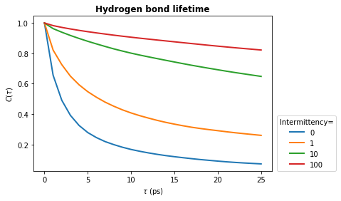
Intermittent lifetime
The above example shows you how to calculate the continuous hydrogen bond lifetime. This means that the hydrogen bond must be present at every frame from \(t_0\) to \(t_0 + \tau\). To allow for small fluctuations in the DA distance or DHA angle, the intermittent hydrogen bond lifetime may be calculated. This allows a hydrogen bond to break for up to a specified number of frames and still be considered present.
In the lifetime method, the intermittency argument is used to set the maxium number of frames for which a hydrogen bond is allowed to break. The default is intermittency=0, which means that if a hydrogen bond is missing at any frame between \(t_0\) and \(t_0 + \tau\), it will not be considered present at \(t_0+\tau\). This is equivalent to the continuous lifetime. However, with a value of intermittency=2, all hydrogen bonds are allowed to break for up to a maximum of
consecutive two frames.
Below we see how changing the intermittency affects the hydrogen bond lifetime.
[12]:
tau_max = 25
window_step = 1
intermittencies = [0, 1, 10, 100]
[13]:
for intermittency in intermittencies:

    tau_frames, hbond_lifetime = hbonds.lifetime(
        tau_max=tau_max,
        window_step=window_step,
        intermittency=intermittency
    )

    times_times = tau_frames * u.trajectory.dt
    plt.plot(times_times, hbond_lifetime, lw=2, label=intermittency)

plt.title(r"Hydrogen bond lifetime", weight="bold")
plt.xlabel(r"$\tau\ \rm (ps)$")
plt.ylabel(r"$C(\tau)$")

plt.legend(title="Intermittency=", loc=(1.02, 0.0))
plt.show()
Hydrogen bond lifetime of individual hydrogen bonds
Let’s first find the 10 most prevalent hydrogen bonds.
[14]:
hbonds = HydrogenBondAnalysis(universe=u)
[15]:
hbonds.run(verbose=True)
[16]:
# Print donor, hydrogen, acceptor and count info for these hbonds
counts = hbonds.count_by_ids()
for donor, hydrogen, acceptor, count in counts[:10]:
    d, h, a = u.atoms[donor], u.atoms[hydrogen], u.atoms[acceptor]
    print(f"{d.resname}-{d.resid}-{d.name}\t{h.name}\t{a.resname}-{a.resid}-{a.name}\tcount={count}")
ARG-71-NH2      HH22    ASP-76-OD1      count=98
TYR-193-OH      HH      GLU-108-OE1     count=97
ARG-2-NH1       HH11    ASP-104-OD1     count=96
THR-199-OG1     HG1     ASP-197-OD1     count=95
TYR-24-OH       HH      GLY-214-OT2     count=95
TYR-133-OH      HH      ASP-146-OD1     count=95
ARG-206-NE      HE      GLU-210-OE1     count=93
ARG-124-NH2     HH22    GLU-143-OE1     count=93
LYS-200-NZ      HZ2     ASP-208-OD2     count=93
LYS-211-NZ      HZ3     GLU-204-OE1     count=92
Now we’ll calculate the lifetime of these hydrogen bonds. To do this, the simplest way is to run HydrogenBondAnalysis for each hydrogen bond then use the lifetime method. It is very efficient to find hydrogen bonds between two specific atoms, especially with update_selections=False.
[17]:
tau_max = 25
window_step = 1
intermittency = 0
[18]:
hbond_lifetimes = []
labels = [] # for plotting

for hbond in counts[:10]:

        # find hbonds between specific atoms
        d_ix, h_ix, a_ix = hbond[:3]
        tmp_hbonds = HydrogenBondAnalysis(
            universe=u,
            hydrogens_sel=f"index {h_ix}",
            acceptors_sel=f"index {a_ix}",
            update_selections=False
        )
        tmp_hbonds.run()

        # calculate lifetime
        taus, hbl, = tmp_hbonds.lifetime(
            tau_max=tau_max,
            intermittency=intermittency
        )
        hbond_lifetimes.append(hbl)

        # label for plotting
        donor, acceptor = u.atoms[d_ix], u.atoms[a_ix]
        label = f"{donor.resname}:{donor.resid} to {acceptor.resname}:{acceptor.resid}"
        labels.append(label)

hbond_lifetimes = np.array(hbond_lifetimes)
labels = np.array(labels)
[19]:
# Plot the lifetimes
times = taus * u.trajectory.dt
for hbl, label in zip(hbond_lifetimes, labels):
    plt.plot(times, hbl, label=label, lw=2)

plt.title(r"Hydrogen bond lifetime of specific hbonds", weight="bold")
plt.xlabel(r"$\tau\ \rm (ps)$")
plt.ylabel(r"$C(\tau)$")

plt.legend(ncol=1, loc=(1.02, 0))
plt.show()
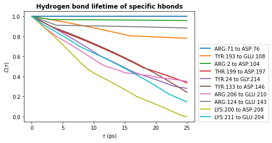
Note
The shape of these curves indicates we have poor statistics in our lifetime calculations - we used only 100 frames and consider a single hydrogen bond.
The curve should decay smoothly toward 0, as seen in the first hydrogen bond lifetime plot we produced in this notebook. If the curve does not decay smoothly, more statistics are required either by increasing the value of tau_max, using a greater number of time origins, or increasing the length of your simulation.
See Gowers and Carbonne (2015) for further discussion on hydrogen bonds lifetimes.
References
[1] Richard J. Gowers, Max Linke, Jonathan Barnoud, Tyler J. E. Reddy, Manuel N. Melo, Sean L. Seyler, Jan Domański, David L. Dotson, Sébastien Buchoux, Ian M. Kenney, and Oliver Beckstein. MDAnalysis: A Python Package for the Rapid Analysis of Molecular Dynamics Simulations. Proceedings of the 15th Python in Science Conference, pages 98–105, 2016. 00152. URL: https://conference.scipy.org/proceedings/scipy2016/oliver_beckstein.html, doi:10.25080/Majora-629e541a-00e.
[2] Naveen Michaud-Agrawal, Elizabeth J. Denning, Thomas B. Woolf, and Oliver Beckstein. MDAnalysis: A toolkit for the analysis of molecular dynamics simulations. Journal of Computational Chemistry, 32(10):2319–2327, July 2011. 00778. URL: http://doi.wiley.com/10.1002/jcc.21787, doi:10.1002/jcc.21787.
[3] Paul Smith, Robert M. Ziolek, Elena Gazzarrini, Dylan M. Owen, and Christian D. Lorenz. On the interaction of hyaluronic acid with synovial fluid lipid membranes. Phys. Chem. Chem. Phys., 21(19):9845-9857, 2018. URL: http://dx.doi.org/10.1039/C9CP01532A
[4] Oliver Beckstein, Elizabeth J. Denning, Juan R. Perilla, and Thomas B. Woolf. Zipping and Unzipping of Adenylate Kinase: Atomistic Insights into the Ensemble of Open↔Closed Transitions. Journal of Molecular Biology, 394(1):160–176, November 2009. 00107. URL: https://linkinghub.elsevier.com/retrieve/pii/S0022283609011164, doi:10.1016/j.jmb.2009.09.009.
[5] Richard J. Gowers and Paola Carbonne. A multiscale approach to model hydrogen bonding: The case of polyamide. J. Chem. Phys., 142:224907, June 2015. URL: https://doi.org/10.1063/1.4922445